User’s Manual
Introduction
Matpower (Matpower) is a Matlab software package being actively developed and maintained by Cornell University researchers and graduate students since 1992. Also, many Matpower users have contributed numerous academic and real life networks data in Matpower Case (MPC) format. It is mature, reliable package for simulation, analysis and optimization of electrical power systems in steady state operations. Since it is written in Matlab scripting language it allows for expansion using all Matlab Toolboxes. There are some other software packages with the same objectives written in other languages but Matlab programming language is still the undisputed programming language used in science and engineering. Matlab is pricey commercial software not affordable by many researches in academia and industry. Fortunately, Matpower also runs under the public domain Matlab clone called Octave (Octave) without any changes. Matpower is the ideal tool for seasoned researchers comfortable using Matlab and knowledgeable of power systems operations but not so useable for students and power systems engineers without Matlab experience. The main difficulties are caused by the lack of Graphical User Interface (GUI). The two main difficulties are editing new MPC cases and visualising the results of Matpower algorithms. The editing of new MPC networks is very error prone and time consuming without being able to see what the network looks like while being edited as well as not being able to examine network items parameters. The second difficulty is with visualising the results of Matpower calculations. While numerical data can be easily examined in Matlab, such approach does not provide qualitative understanding of network operations. Because of these issues, Matpower is used with power network data converted from other packages like PSSE and PowerWorld to MPC. Matpower installation comes with a very large collection of very small to quite large networks in MPC format converted from other, mostly commercial, packages. To rectify these problems, Bia Soft developed Matpower Viewer or MPV for short.
MPV is a power systems network editor and viewer similar to PSSE and PowerWorld. It does not provide any computational algorithms but it interfaces with Matpower to provide it with networkd data and to get the results back to display. The interface with Matpower, running in either Matlab or Octave, is done using MPC files. It is possible to fully integrate MPV with Matpower as a single program but with some difficulty. Interfacing MPV and Matpower through a file allows MPV to be customized to be used with other similar programs. This interfacing method allows for interfacing with both commercial and non-commercial applications.
MPV is developed using libraries with licenses permissible for commercial use but MPV itself is a commercial product. MPV was developed without any academic or government support and cannot be further developed or maintained without charging a minimal fee for it. Will MPV ever be released to public domain? It probably will when it is mature enough and there are volunteers interested in taking over the development and maintenance.
Currently, MPV runs on x_86 64 bit hardware under Windows, Linux and MacOS. Also, MPV runs well on Apple Silicon computers with Rosetta 2 installed. MPV is designed to be as intuitive and flexible as possible so this User’s Guide is just an overview of its features and capabilities. Anyone who has used similar engineering software previously will be comfortable with MPV within minutes. It is possible to run MPV and Matpower in parallel, that is, perform calculations in Matpower and sync the results from MPV but it should be done carefully since MPV’s flexibility allows for different unintended scenarios. Good familiarity with the Matpower data format and its basic algorithms is assumed.
Installation
MPV is supported on Windows, Linux and MacOS operating systems. On Windows and MacOS installation programs require Administrator or root privileges. If not having administrative privileges shows to be a problem, portable versions will be compiled and provided. MPV does not depend on system resources such as registry. Linux installation is more flexible allowing to specify installation directory which could be in user’s personal space. On Windows and MacOS MPV is run by double clicking on its icon or from the command line if the executable (app in MacOS case) is in $PATH. On Linux it can be done by double clicking on the desktop icon or from the command line. If it is run from the command line, it must be started from the installation directory. To start from any other directory, create a function to switch to the installation bin directory and run MPV. As an example for bash, add to .bashrc and/or .bash_profile after adjusting the path of MPV executable:
function MPV() {
   pushd . >/dev/null
   cd /home/user_name/mpv/mpv-1.2.0.0/bin
   ./mpv-1.2.0.0 &
   popd >/dev/null
}
User can also put installation bin directory in $PATH but in that case installation library path must be added to $LD_LIBRARY_PATH. Some Linux distributions, like newer Ubuntu versions, make it almost impossible to modify $LD_LIBRARY_PATH without root privileges. Note that while both the commercial and free versions can be run as a portable application from a USB drive, the commercial version is tied to a particular computer’s hardware and can be run only on the computer on which it is registered.
More information can be found on the Downloads page.
Editing
The Matpower data can be in textual (*.m) or binary (*.mat) format. MPV uses *.mat binary format to preserve binary accuracy and to avoid matlab executable code in *.m script interpretable by Matlab or Octave only. While the code in *.m file can be ignored and only relevant data extracted from the mpc structure, the code could modify the data and MPV could read wrong data depending on what the script part does. A *.mat file must contain a Matpower structure named mpc with at least mpc.version, mpc.baseMVA, mpc.mpc.bus, mpc.gen and mpc.branch structure elements. In addition to these components, Matpower users can and have used additional information for their specific needs. MPV also allows for mpc.dcline, mpc.bus_name, mpc.gentype and mpc.genfuel. The last three mpc structure data types are cell arrays with text elements either UTF-16 or UTF-8 encoded depending whether defined in Octave or Matlab. Octave officially uses UTF-8 encoding. Matlab internally officially uses UTF-16 or UTF-8 depending on the version. Matlab version R2016b and earlier uses ASCII which is compatible with UTF-8, R2017a-R2020a uses UTF-16 and R2020b and later uses both UTF-16 and UTF-8. Unfortunately, MPV cannot reliably detect and use UTF-16 encoding. Specifying option -v6 or -v7 when saving *.mat files seems to use UTF-8 or ASCII format which is compitable with MPV. If there are problems with the text encoding, make sure to specify option -v7 when saving *.mat files to be read by MPV. Note that character encoding affects mpc cell arrays only if used at all.
Additional data types and power systems device models can be added on request. Matpower and Matlab are very flexible number crunching environments and additional devices like FACTS could be added without much effort if there is interest. Future MPV versions will probably include additional data for dynamic simulators based partially on Matpower data. One of the issues with Matpower data format is that in some situations there are parallel elements that are difficult to distinguish between. For example, there can be multiple generators on a bus with associated generation cost functions and Matpower algorithms depend on matching their ordering in mpc matrices. Also, there can be parallel lines between buses which is less of an issue. In addition to usual mpc data described in Matpower User’s Manual, MPV uses labels for buses, generators and branches. These labels are used by MPV internally and for displaying. Labels are assigned automatically and can be modified manually by the user and can be ignored except generator labels. If there are multiple generators attached to a bus they all must have a unique label at that bus. MPV network can be entered from:
scratch
a Matpower file *.mat manually or
a mat file automatically
Edit From Scratch
Entering a new network from scratch is similar to other commercial applications like PSSE and Powerworld. MPV provides a way to visually enter all the usual Matpower elements but it also adds some additional information to distinguish between multiple generators and branches. These additional information is optional and it is safe to use default values provided by MPV. An mpc network is entered using a series of dialogs:
Add Bus: To add a bus left click on the bus icon on the toolbar and then left click on the canvas where you want the bus to be placed. A dialog box pops up to enter parameters. Some entries in the dialog box are disabled and grayed out because they are output values or should not be modified. Repeat this to enter all the buses you want.
Add Generator: To attach a generator to a bus, left click on the generator icon on the toolbar and then on the bus. A generator dialog will pop up to enter generator parameters. Note that the first generator entered defines the cost function model and if there is reactive power cost. Both real and reactive power cost curves must be of the same model and with the same number of function coefficients or points in the case of piecewise linear (PWL) functions. There is limited flexibility in shaping the cost functions through function coefficients or points in the case of PWL functions. For example, if model is specified as a quadratic function, setting the the quadratic term coefficient to zero results in a linear function. Note that all cost functions should be convex.
Add Shunt or Load: To attach a shunt or load to a bus, left click on the shunt or load icon on the toolbar and then on the bus. Since load and shunt are part of mpc.bus record the bus dialog pops up allowing to modify load or shunt values only. Shunt or load image will not be displayed for zero shunt or load. To add shunt or load image with zero value set shunt or load to a non-zero value when entering it and change it afterwards to zero and the image will remain displayed.
Add Branches, Transformers, DC Lines: To connect two buses with a branch, transformer or a DC line, left click on the item on the toolbar, then left click on the from bus and then on the to bus. A dialog box pops up to allow you to enter parameters.
Add a Label: RIGHT CLICK on an item pops up a dialog to associate and display a label for that item. An item’s label can be moved around the item but it is restricted to it’s vicinity. RIGHT CLICK on branch, transformer or DC line will pop up a dialog to choose a label type, insert a connector on the line or in the case of a plain branch to toggle it between a simple branch and transformer.
Add a Branch Connector: Branch connectors are used to display a branch in segments. A connector can be placed on a branch with RIGHT CLICK on a branch. Selecting that branch with LEFT CLICK will highlight all the connectors. Select again just the connector to be moved and display branch in segments.
Resizing Buses: Sometimes there can be multiple generators on a bus making it difficult to display them all. In such situations the bus can be made longer (or shorter) by selecting the bus and pressing CTRL and ← to shorten or → to make the bus longer. This operation can be applied to multiple selected buses at the same time. If the network is very large, make buses very short with no elements connected to display just the network topology and maybe the power flows.
Fine Positioning: For fine positioning select one or multiple items with CTRL+LEFT click. Single or multiple selected items can be moved in small steps with ALT + ←,↑,→,↓ and aligned them with the grid. This is especially convenient when preparing high quality network images for publications.
Selecting Multiple Items: Multiple items can be selected one by one using CTRL+LEFT and slicking on each item or by defining a rubber band area using CTRL+LEFT click in empty area and moving around until all desired items are selected. After all desired items are highlighted, all operations applicable to a single item can be applied to the highlighted items.
Toggling The Background Grid: RIGHT CLICK in empty space on the canvas pops up a menu to toggle background grid.
Item Orientation: Item icons and labels can be flipped and rotated using the toolbar.
Editing Entered Items: After the entire or part of the network is entered any existing item’s parameters can be modified by double clicking left mouse on the item and editing the parameters. Note that branches are not independently movable but an entire branch or just a segment can be moved by selecting and moving connectors. To move a connector select a branch and all its connectors will be highlighted. Left click on a connector will choose just that single connector which will allow you to move it around and shape branch path.
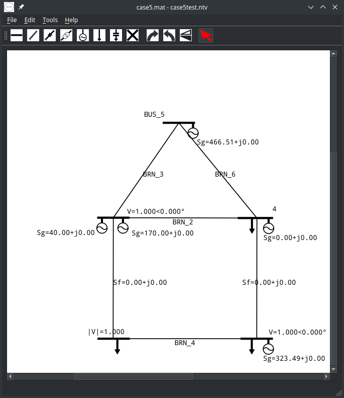
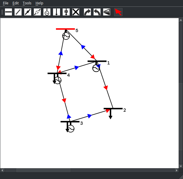
Figure of the case5.mat network from the Matpower archive as an example. Entering this small network takes considerably more time than by importing case5.mat or using automatic layout method explained later.
Editing From MPC File
MPV can use a Matpower *.mat file with mpc structure as a starting point to produce a visual representation of the network described in the mat file. To do this, user first imports a *.mat file by clicking on the menu entry File->Import and selecting *.mat file with the network to import. This will read the mat file into memory where it can be used for displaying or modifying by the user through MPV dialogs. The MPV editing process is very similar to a starting from scratch approach except that the user is also presented with available and applicable network items from the mat file in a drop down list. Attention must be paid when choosing branches from the drop down list. If you need to enter an I to J branch not on the list of available branches for this pair of nodes, check if the J to I branch is. It is easy to enter extra parallel branches by mistake.
In this example, the mpv network is built starting from case5.mat from Matpower case archive.
When entering a new bus, the “Display Devices” box can be checked to display other devices (shunt and load) attached to the bus if there are any. A device is present if its parameter is non-zero. If a device parameter is zero it will not be displayed even if “Display Devices” box is checked. If a device with zero parameter is to be displayed it can be done by adding it with a non-zero parameter using the toolbar and then change the parameter value to zero after double clicking on it. Adding a branch from the *.mat file follows scratch method steps except that the branch can also be chosen from the drop down list. If the branch is not available in the drop down list but it should be, you probably reversed to-from buses.
MPV allows editing and viewing an entire Matpower network or just a part of it. When a mat file is imported and part of it is modified through MPV, the entire file with the modification is saved, not just the parts displayed in MPV when saved from MPV File menu.
Since not all the elements from *.mat file have to be displayed, when deleting an element on the canvas, the user is given an option to delete just the GUI symbol or both the GUI symbol and the associated data imported from the *.mat file. If a bus item is deleted, all the items connected to that bus are deleted either just from the canvas or from the canvas and data store. If an item is deleted from the canvas only, it is available to place it on the canvas again.
Automatic Layout
Entering a Matpower network into MPV manually can be time consuming even if it is done using data from a *.mat file because it is difficult to arrange items in a “visually pleasing” graph. Once all the buses and branches of interest are positioned on the canvas, buses need to be arranged and branches possibly rerouted. This task can be quite time consuming. To help with this, MPV can automatically import a *.mat file and arrange the buses and connect the branches. This is by no means perfect since visually pleasing layout is subjective criterion but it does help with rearranging buses and rerouting branches manually.
Automatic Layout dialog is started from the menu with Tools->Automatic Layout and consists of four parts: Display Items, Layout Algorithm, Layout Parameters, and Network Layout.
Display Items defines what network items to display with the layout. Buses, branches and DC-lines are always displayed but other items do not have to be displayed. If the network is very large it might be better to display the buses and branches only and maybe even reduce bus sizes as explained later.
Layout Algorithm selects the algorithm to be used to position buses. Two different automatic layout algorithms are available. One, called Repel Method in the layout dialog, uses the classical spring repelling force algorithm while the second, Attract/Repel Method, uses repeling forces between non-adjacent nodes and attracting force between adjacent nodes. The first method is better for smaller networks and second method is more appropriate for larger networks. The Repel Method parameters are the Maximum Iterations and the Maximum Node Energy. Increasing Maximum Iterations should result in lower Maximum Node Energy. Termenating number of iterations and maximum node energy is shown in the lower left corner on the status bar to help with adjusting these parameters. The Attract/Repel automatic layout algorithm allows for islands and shows them isolated so it is easy to visualize if the network is disconnected or weakly connected. There are two pairs of parameters that affect this layout and the user can adjust them by going to the Tools->Automatic Layout menu. It takes a little bit of practice adjusting these parameters to get good layouts that need small manual editing even for large networks. Both methods depend on the size of the area used to display the network. This area should be smaller than the main window size defined in the Preferences dialog. If, with Attract/Repel method, items are pushed to the edges of the area defined with X,Y,W and H settings attraction should be increased and repulsion reduced or a combination of the two used. Similar adjustments should be applied if items are positioned too far away from all the edges. The entire network or just a part of the network can be displayed by either method as defined by Network Layout part of the dialog. Note that the Repel Method cannot handle networks with islands.
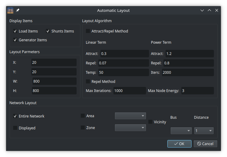
Layout Parameters specify layout position and size. X,Y is the upper left corner which is the graph origin and W and H are the width and height of the display area measured to the right and down from the origin respectively. X,Y,W,H define the graph display area and must be smaller than the main window size set in the Preferences dialog. Both layout algorithms are sensitive to the layout size and it should be adjusted along with the rest of adjustable layout parameters.
Attract/Repel Parameters are applicable to the Attract/Repel algorithm only. Attract/Repel Parameters are linear and power coefficients used to calculate attraction and repulsion forces used by the placement algorithm. Attraction forces are between adjacent buses and repulsion is between non-adjacent. Manipulating these forces different network features like islanding and weak connectivity can be revealed. Parameters Temp and Iters specify search speed and maximum number of iterations to use.
Reppel Parameters Maximum Iterations and Maximum Node Energy define algorithm termination. If the current iteration number is equal to Maximum Iterations or the current maximum node energy is less or equal to the Maximum Node Energy parameter the algorithm terminates. Terminating number of iterations and node energy are shown at the left side of the status bar and can be used to adjust them in subsequent runs.
Automatic layout can display all the buses and connecting branches, some or none. The used placement algorithm starts from a random arrangement and can result in different final placements at each run. Run multiple times and with different parameters if not satisfied with the final arrangement. Use menu Tools->Automatic Layout dialog to explore different possibilities.
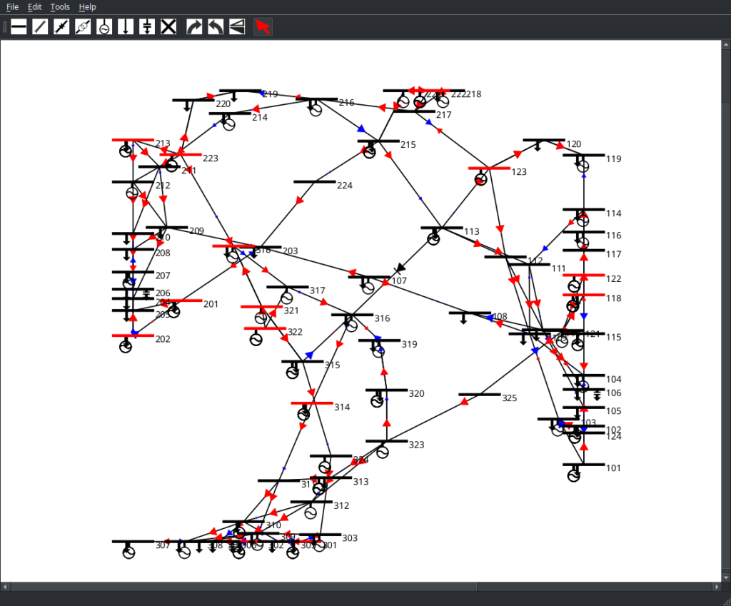
Automatically laid out case_RTS_GMLC which consists of three 24 bus networks. Bus numbers start with 1, 2 and 3 for each of the sub-networks. These three networks are grouped almost completely separately due to loose connections between and can be easily identified on the layout below.
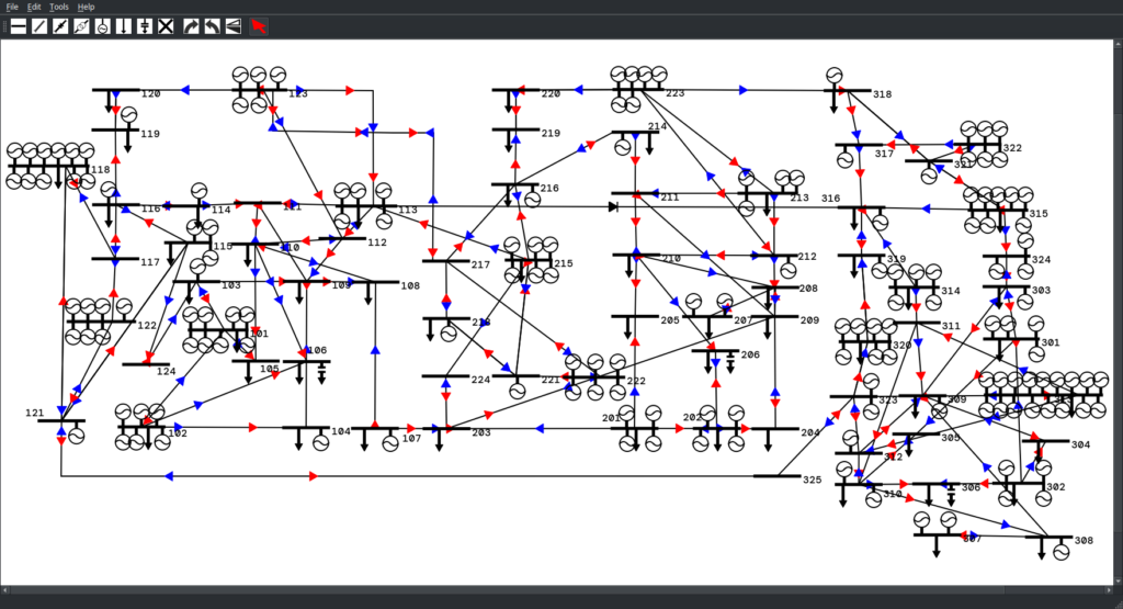
Resulting layout after 10 minutes of rearranging it manually. Note that in the automatic layout the multiple generators on buses were overlapping and had to be separated manually. Multiple generators and branches overlap by default to minimize the number of visible generators and branches while keeping the connectivity representation but it could be a settings in future versions.
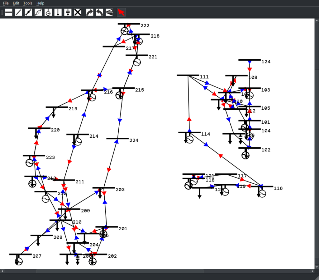
Automatic layout after adjusting layout parameters, removing one of the areas and disconnecting the remaining two from each other.
Network Layout part of the dialog specifies what parts of the network to layout and display. MPV can layout the entire network, particular area or zone, vicinity of a bus or layout the displayed part of the network again. The dialog enables or disables applicable options. For example, if Repel algorithm is checked all Atract/Repel parameter options are disabled. Similarly, only one of Entire Network, Displayed, Area, Zone or Vicinity can be checked. While other Network Layout options are self explanatory, Vicinity options needs some explanation. Vicinity layout is used by choosing a Bus and Distance. Bus is the bus whose vicinity we want to explore and Distance is the maximum number of branches connecting to nearby buses. Bus drop down list lists all the buses in the network and Distance is limited to at most ten branches. Laying out vicinity of a bus is computationally intensive.
Viewing
MPV display is highly configurable. Going to menu Edit->Preferences opens a dialog allowing to choose the default settings that are preserved between MPV runs. Changing some of the settings will take effect immediately and some on the next run. For some of the settings, these are just the default values that can be changed on per item case.
Edit->Preferences dialog consists of two tabs and allows for detailed display configuration.
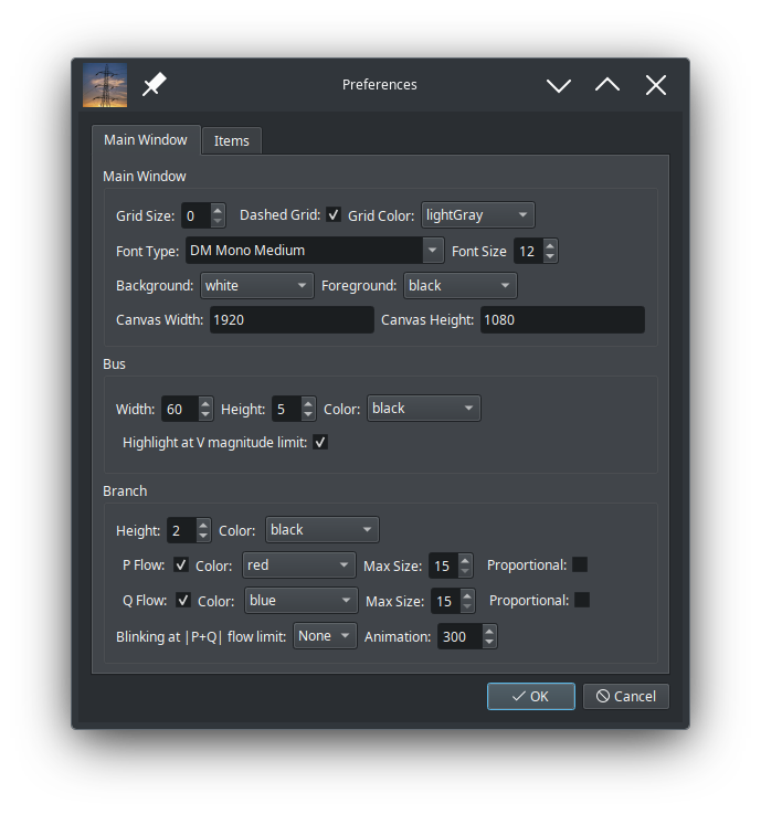
Main Window settings define default values for font type, font size, colors and grid density and canvas size can be specified.
Bus part of the dialog sets default bus size and color and whether the bus is highlighted red if the voltage magnitude is at or outside the limits.
Branch options in addition to branch size and color also include the P Flow and Q Flow settings. If P Flow and/or Q Flow are checked branches will display arrows in the power flow direction and using the color specified in Color fields. Max size field specifies the maximum size of the arrow and Proportional check box if the arrow is to be scaled with respect to the apparent power flow magnitude. If the Blinking at |P+Q| flow limit checkbox is enabled, the arrow will blink if the specified limit is reached at intervals given in Animation field in milliseconds. If this value is zero arrows will not blink.
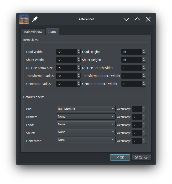
Items preferences tab specifies other items sizes and default labels. For numerical labels, accuracy (number of digits after the decimal point) can be specified here.
GUI Viewing
MPV networks can be displayed well on different resolutions and multiple screens including high DPI with zooming in and out. A single item cam be moved around by selecting it and moving it with the left mouse button.
Zooming: Zoom in with + and zoom out with –
Grid Toggle: Press RIGHT CLICK in empty area on the canvas to toggle background grid lines.
Panning: Press SHIFT + LEFT BUTTON and move the mouse to pan.
Moving Group of Items: Moving groups of items: Select a group of items either by enclosing them with a rubber band, CTRL+LEFT CLICK + mouse move, or selecting them individually with CTRL+LEFT CLICK on each item. LEFT CLICK on one highlighted item and move it around and all highlighted items will follow.
Table Viewing
MPV can show two different representations of the same network, one is GUI and the other one is tabular. Menu Tools->Edit MPC opens a tabular view of the network. The following two pictures show the two representations of the modified case5 network.
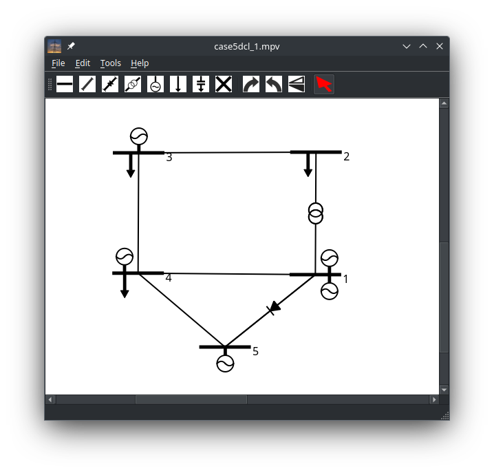
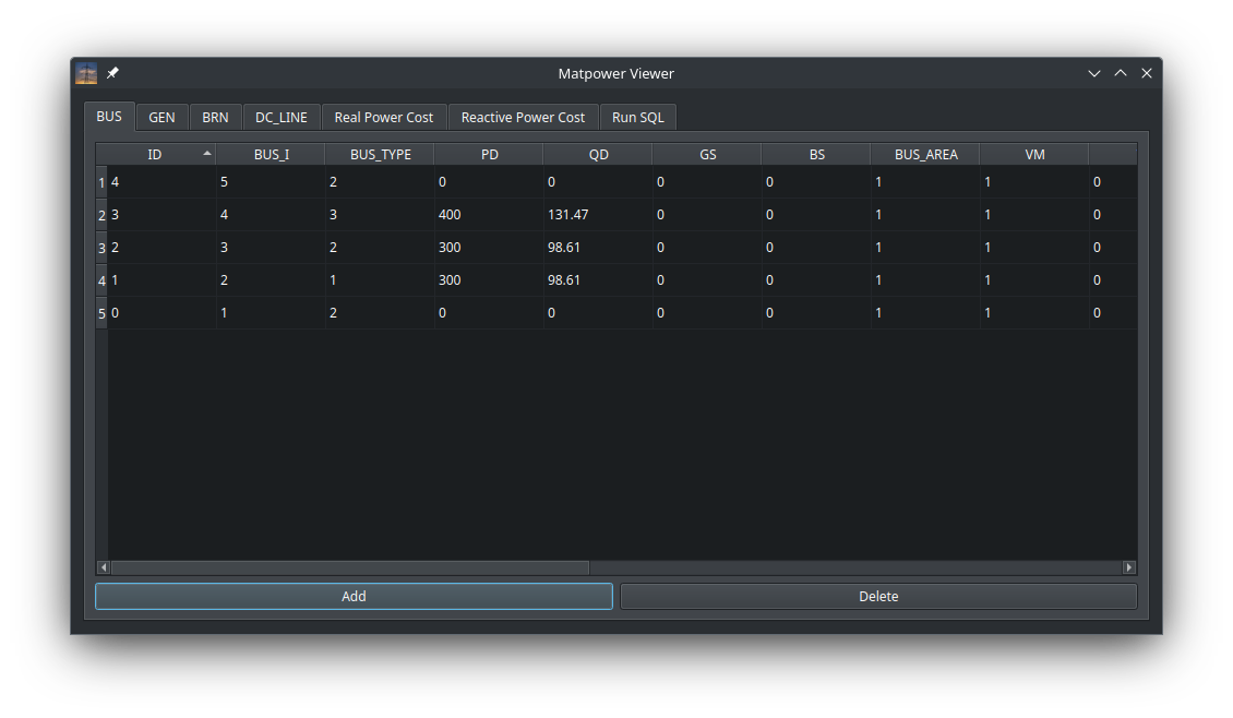
In the tabular view, network items can be viewed, edited, added and deleted. Not all the fields are editable, just like in the GUI view. For example, fields that are results of a calculation are not editable. Also, some fields, like bus number, should not be modified after defined for the first time. The most obvious example are the real and reactive power costs. The first generator entered defines the cost model and how many parameters all the subsequent cost functions must have. The first generator also determines if reactive power cost functions are used or not. Tabular viewing and editing method is appropriate for entering large networks because it does extensive consistency checking that would be tedious to do in Matlab or Octave. Networks can be entered, saved and exported to either *.m or *.mat files without using the GUI representation at all.
Items can also be deleted in the tabular view. If an item with attached items is deleted the attached items are deleted as well if it does not make sense to keep them. If a deleted item is also in the GUI view, the deletion is reflected immediately in the GUI view as well. Deleting items in Matpower is especially error prone while in MPV it is not a problem a at all.
Tabular view also provides a Run SQL tab. User can perform complex searches in this tab but the network cannot be modified using SQL statements. Basically, only SELECT statements are allowed.
Note that the tabular view is a modal dialog so the GUI view cannot be accessed until the tabular view is closed. Changes made in the GUI view are reflected in the tabular view when the tabular view is opened again.
Loading And Saving
An MPV network can be saved to and loaded from an *.mpv file. A *.mat file can be used as the starting point for entering and displaying a network. A displayed network can also be exported to a *.mat file. The MPV file is an extended SQLite database. If it is more convenient to explore and edit tables than using dialogs, there are many SQL management public domain programs to do so. SQLiteStudio is just one of them available for Windows, Linux and MacOS. Remember that editing MPV files using external tools will not ensure network consistancy. An mpv network can be exported to *.mat, *.m Matpower data files or to a *.png image file. Editing MPV SQL file directly can corrupt it if GUI records are edited or deleted or bus records are deleted without deleting attached branches or generators. Following is the list of usual input and output operations:
Start New mpv file: Menu File->New erases current mpv file and starts a new one.
Load mpv File: Select Menu File->Open to open an existing mpv file.
Save and Save As mpv File: Use File->Save or File->Save As to save or save as the current mpv file.
Export as *.m, *.mat or *.png file: File->export allows you to choose mpv file export format and to export it.
Syncing with *.mat file: Tools->Sync syncs a *.mat file with the current mpv file.
Here are some examples of loading and saving case5a.mpv and export operations and their results:
And resulting exported case5a_test.m file:
case5a_test.mat file viewed in Octave:
and case5a_test.png viewed in gwenview on Linux:
Integrating With Matpower
MPV can be run in parallel with Matpower. The user can enter or modify an mpv file, export it to a mat file, read it by Matpower and perform desired operations on that mat file. When all the desired operations are performed, the mat file can be synced with MPV and the results displayed. Note that MPV can use the entire or part of the mat file while Matpower uses the entire mat file. Syncing with a Matpower file is not the same as importing that Matpower file. Syncing with a Matpower file reads *.mat file and updates data associated with the displayed items while importing a Matpower file just reads the *.mat data and does not display any items. Syncing can be done multiple times from the same or different *.mat file which can be very useful but must be done carefully.
Here is an example how this can be done:
Note that voltage magnitude of the bottom right bus increased as the real demand on the same bus was changed from 300MW to 100MW. Real power flows from bus, Pf, changed as well. This is due to running the power flow after changing the demand. Although syncing allows for some interesting multiple runs and network analysis with different configuration and settings, it is important that items in mpv file being synced and mat items synced with exist, otherwise the results are undefined or MPV could also crash.